Bayesian Updating with INLA
Mar 24, 2018Online Updates
Machine Learning involves adjusting the weights of a model based on data, so that the model becomes increasingly better at approximating some desired function. Some ML models are easy to update “online,” while deployed. Other times, batch training is the only practical option.
Way before people started using that term, though, it was easy to do “online learning” with a Bayesian model. The old posterior distribution for the model parameters becomes the new prior. Often people forget to mention this important fact about priors when introducing them to beginners—They’re often based on previously digested data!
Getting the posteriors
In a call to the inla R function, the coefficients have Gaussian prior. By default it’s very wide, so the data gets to influence the posterior maximally. If the latest batch of data isn’t that big a deal compared to what you’ve seen before, though, the new data should only refine, not define, the model.
Let’s create the same extremely simple model as last time. INLA handles a wide variety of models, but the usage doesn’t change much, and using the same one is hopefully less distracting.
library(INLA)## Loading required package: sp## Loading required package: Matrix## This is INLA_17.06.20 built 2018-03-14 23:31:50 UTC.
## See www.r-inla.org/contact-us for how to get help.set.seed(1)
inla.seed = 2
x <- 1:100
y <- 5 + 4 * x + rnorm(n=length(x), sd=3)
m1 <- inla(y ~ x, data=data.frame(x, y), control.compute=list(config=TRUE))
m1$summary.fixed[,-7]## mean sd 0.025quant 0.5quant 0.975quant mode
## (Intercept) 5.395015 0.546538406 4.319566 5.394999 6.469311 5.395015
## x 3.998646 0.009395883 3.980158 3.998646 4.017115 3.998646Some utility functions will help use these posteriors for the coefficients as priors in the next update to the model. The priors have to be specified with precision, not standard deviation, so the second function makes the conversion.
posterior.mean <- function(m, name) m$summary.fixed[name, "mean"]
posterior.prec <- function(m, name) 1/m$summary.fixed[name, "sd"]^2
Now we prepare to use the “fixed-effects” posteriors from m1 as priors for m2.
fixed.priors <- list()
fixed.priors$mean = list()
fixed.priors$prec = list()
for (name in c("(Intercept)", "x")) {
    fixed.priors$mean[[name]] <- posterior.mean(m1, name)
    fixed.priors$prec[[name]] <- posterior.prec(m1, name)
}
We’ll get around to the noise term soon.
Here’s some new data. There’s not as much as we’ve seen already, but it’s still data, carrying additional information. It is expected to help the model to hone in on the true values, \((5, 4, 3)\).
x <- seq(from=1, to=100, by=5)
y <- 5 + 4 * x + rnorm(n=length(x), sd=3)
The prior for the hyperparameter of m2 requires a bit more thought. We can see right skew, and we know it should have no density left of zero (as a Gaussian would).
library(brinla)
bri.hyperpar.plot(m1)
## Loading required package: ggplot2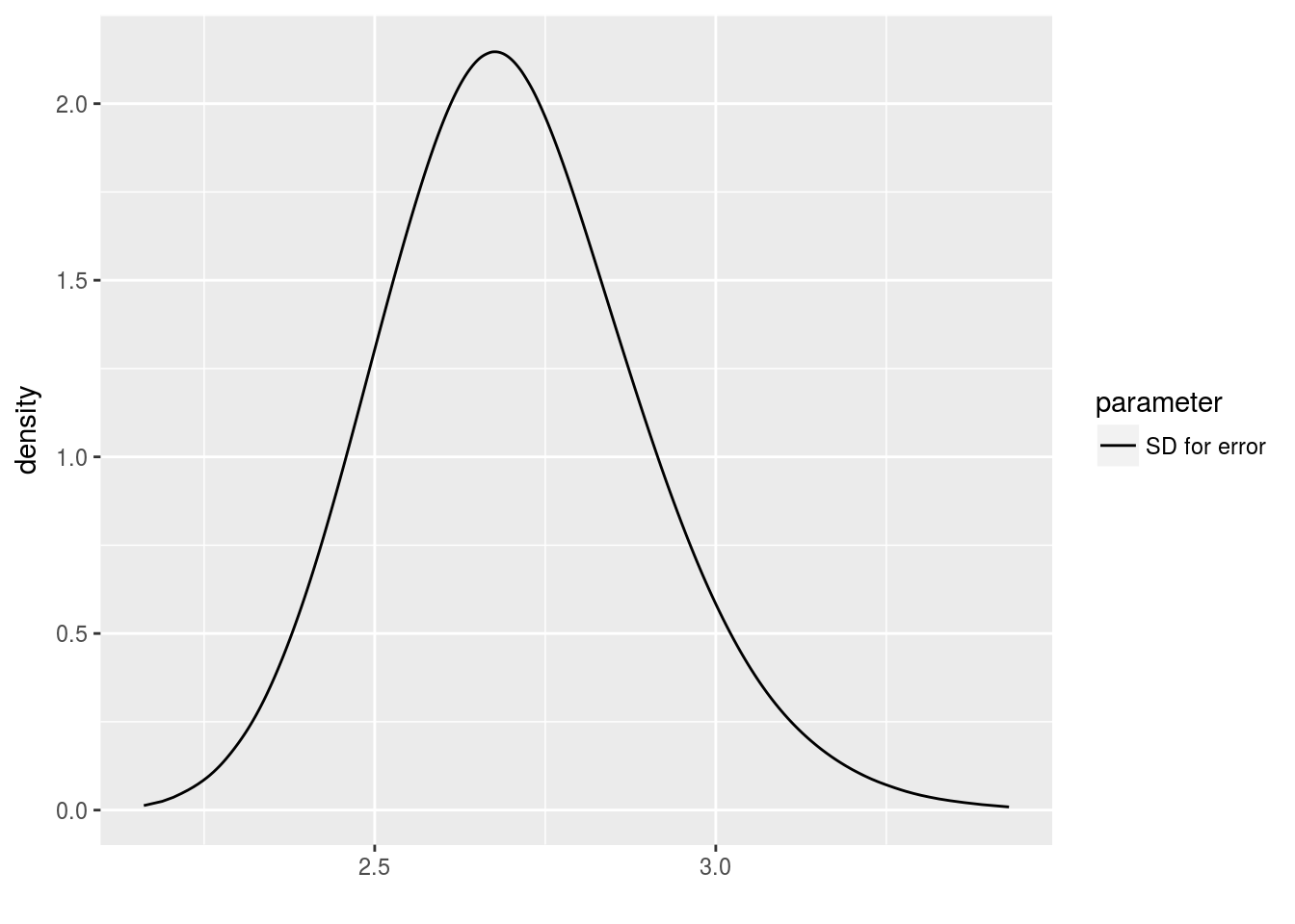
INLA supports several ways to specify the prior for a hyperparameter. It’s surprisingly flexible. One way is to specify a bunch of \(xx\) and \(zz\) points as a way of helping the model approximate a function \(f\) that links them by \(zz = f(xx)\). The \(zz\) here is the log density of the corresponding \(xx\).
Because you can (quickly) sample from the posterior, those points are easy to get.
n.sim <- 100
sim <- inla.posterior.sample(n.sim, m1)
xx <- unlist(lapply(sim, function(s) s$hyperpar))
zz <- unlist(lapply(sim, function(s) s$logdens$hyperpar))
# XXX: Are these xx values "internal scale", as the table requires?
table.string <- paste(c("table:", xx, zz), collapse=" ")
I’m glad that can be automated.
Finally we’re ready to update the model.
m2 <- inla(y ~ x,
    data=data.frame(x, y),
    control.fixed=fixed.priors,
    control.family=list(hyper=list(prec=list(prior=table.string))))
What happened?
That’s not right! The estimates for the true value of the noise got worse, farther from the true value of three. I think that the documentation for the table: feature contained a word that is important. The table requires “internal scale” values of xx, and I’ve used the wrong scale.
d1 <- data.frame(bri.hyper.sd(m1$marginals.hyperpar[[1]]))
d2 <- data.frame(bri.hyper.sd(m2$marginals.hyperpar[[1]]))
d1$model <- 1
d2$model <- 2
d <- rbind(d1, d2)
d$model <- factor(d$model, levels=1:2)
ggplot(data.frame(d), aes(x, y, color=model)) +
        geom_line() +
        ylab("density")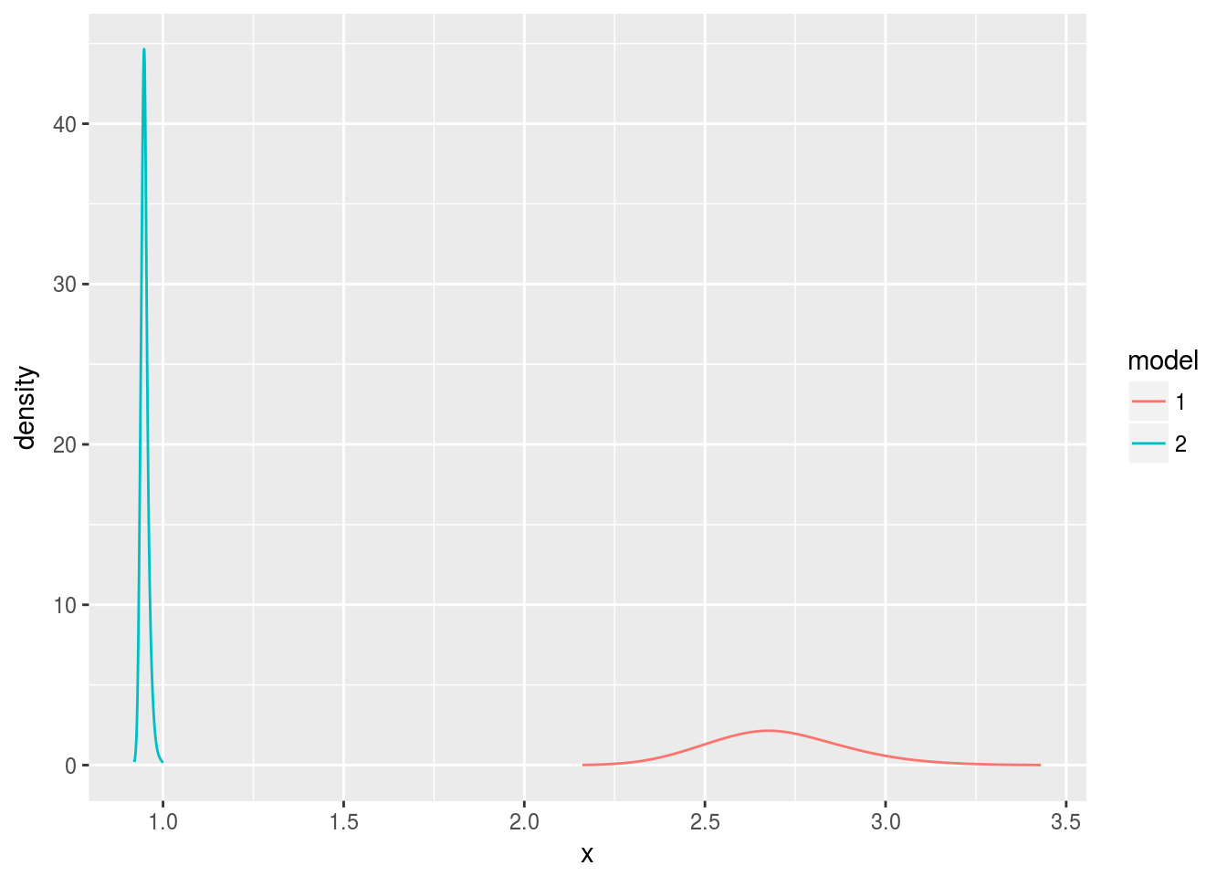
OK. I’ll use the internal values.
str(m1$internal.marginals.hyperpar)## List of 1
## $ Log precision for the Gaussian observations: num [1:75, 1:2] -3.26 -3 -2.74 -2.62 -2.49 ...
## ..- attr(*, "hyperid")= chr "65001|INLA.Data1"
## ..- attr(*, "dimnames")=List of 2
## .. ..$ : NULL
## .. ..$ : chr [1:2] "x" "y"ih <- m1$internal.marginals.hyperpar[[1]]
table.string <- paste(c("table:", ih[,"x"], ih[,"y"]), collapse=" ")
m3 <- inla(y ~ x,
data=data.frame(x, y),
control.fixed=fixed.priors,
control.family=list(hyper=list(prec=list(prior=table.string))))
d3 <- data.frame(bri.hyper.sd(m3$marginals.hyperpar[[1]]))
d3$model <- 3
d <- rbind(d1, d3)
d$model <- factor(d$model, levels=c(1, 3))
ggplot(data.frame(d), aes(x, y, color=model)) +
geom_line() +
ylab("density")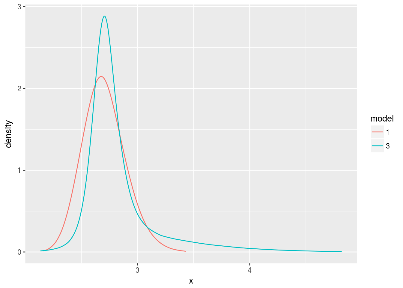
That’s more like it! The posterior of model three (correct updating) is tighter, reflecting the model’s decreasing uncertainty about the parameter, and its mode is closer to three, the true parameter.
Let’s check out the change in the estimates for the fixed parameters as well.
get.fixed <- function(m, model.name) {
    d <- data.frame()
    for (param in names(m$marginals.fixed)) {
        dd <- data.frame(m$marginals.fixed[[param]])
        dd$param <- param
        d <- rbind(d, dd)
    }
    d$model <- model.name
    d
}
d <- rbind(get.fixed(m1, 1), get.fixed(m3, 3))
d$model <- factor(d$model, levels=c(1, 3))
ggplot(d, aes(x=x, y=y, color=model)) +
    geom_line() + ylab("density") + facet_wrap(~ param)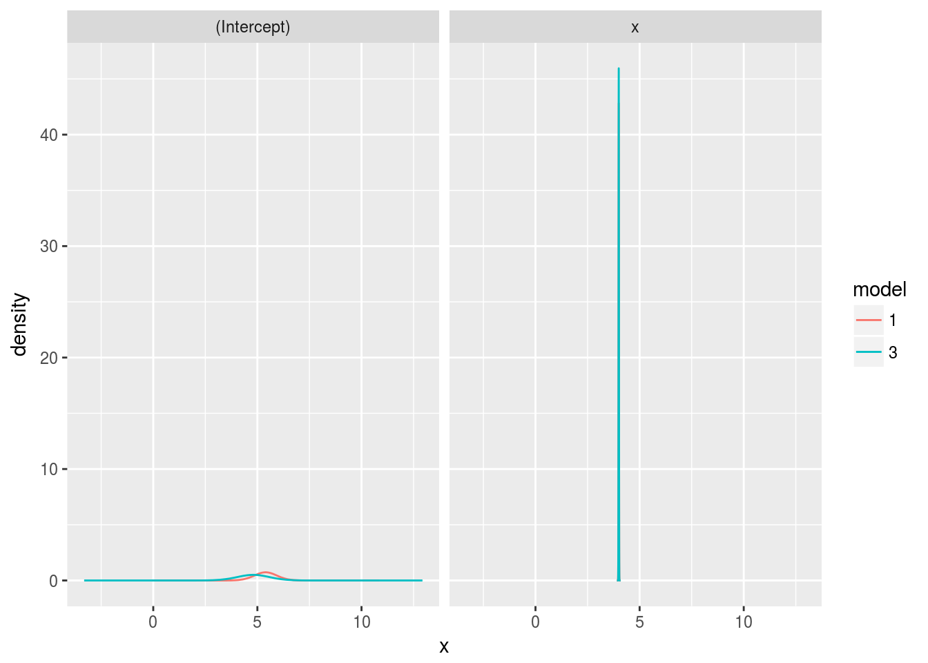
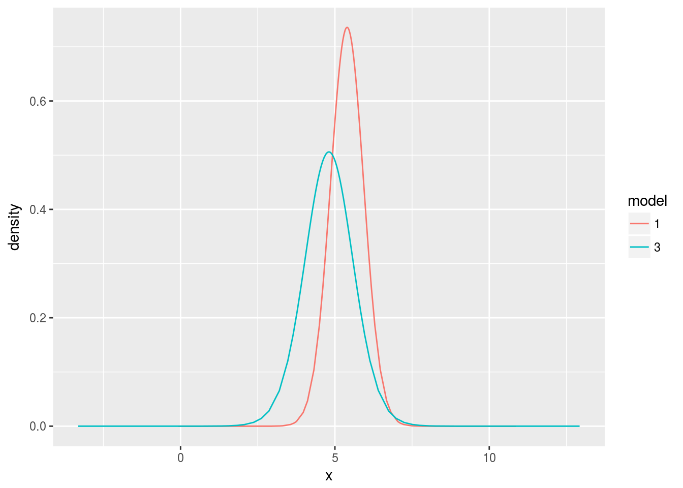
The model was already sure about \(x\), but the estimate for the intercept did improve from updating the model. It’s worth zooming in on the intercept.
library(dplyr)##
## Attaching package: 'dplyr'## The following objects are masked from 'package:stats':
##
## filter, lag## The following objects are masked from 'package:base':
##
## intersect, setdiff, setequal, unionggplot(d %>% filter(param != "x"), aes(x=x, y=y, color=model)) +
geom_line() + ylab("density")